Why Cardinality Estimates Go Wrong: An Oracle Optimizer Lab with Skewed Data

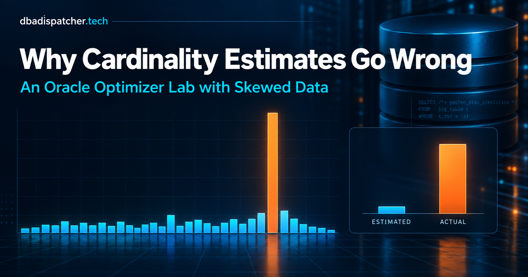
Every Oracle DBA has had this conversation with a developer: "the query ran fine yesterday, it's slow today, nothing changed." Nine times out of ten, when you pull the plan, the root cause is the same one-line diagnosis the optimizer's row estimate for some step is wildly off from what actually came back. E-Rows says 200,000. A-Rows says 4. Everything downstream of that step the join method, the join order, whether an index even gets used was built on a guess that was wrong from the start.

The fix is usually "add a histogram," and that's often right. But "add a histogram" is a reflex, not an understanding, and it doesn't cover every way an estimate goes wrong. I wanted to actually see the failure modes side by side instead of pattern-matching from memory, so I built a small, disposable lab: one table, three different flavors of skew baked in on purpose, and a repeatable way to put the optimizer's estimate next to the truth.

This post walks through what I built and what it showed. Everything here targets 12c/19c and runs fine on Standard Edition 2, nothing needs the Diagnostic or Tuning Pack.

The one trick that makes this whole exercise possible

Before the lab itself, the single most useful technique here is how to get a real actual-row-count next to the optimizer's estimate, in one shot, without touching AWR:

SELECT /*+ gather_plan_statistics */ COUNT(*)
FROM   (SELECT * FROM my_table WHERE some_column = 'RARE_VALUE');

SELECT * FROM TABLE(DBMS_XPLAN.DISPLAY_CURSOR(NULL, NULL, 'ALLSTATS LAST'));

Two things make this work correctly, and both are easy to get wrong:

Wrap the query in COUNT(*). DBMS_XPLAN.DISPLAY_CURSOR's A-Rows column only reflects rows the client actually fetched. If you run a plain SELECT * and your tool only displays the first page of results, A-Rows silently under-reports you'll think the estimate was closer than it was. Wrapping in COUNT(*) forces the aggregate to pull every row from its child row source before it can return anything, so A-Rows on that child line is always the true count.

Read the right line. The top SORT AGGREGATE line will always say A-Rows = 1 one row, the count itself. The number you actually want is on the TABLE ACCESS FULL or INDEX RANGE SCAN line underneath it. This trips people up constantly.

With that out of the way, here's the lab.

Building a dataset with skew you can actually reason about

I generated one table, LAB_ORDERS, with 1,000,000 rows and three independent skew patterns, using a deterministic row generator (MOD/DECODE on the row number, no dependency on external data) so the exact percentages are reproducible run to run:

CREATE TABLE lab_orders (
  order_id      NUMBER        NOT NULL,
  order_status  VARCHAR2(20)  NOT NULL,   -- frequency skew, 5 values
  region_code   VARCHAR2(10)  NOT NULL,   -- looks uniform...
  channel       VARCHAR2(10)  NOT NULL,   -- ...but is correlated with region_code
  order_amount  NUMBER(10,2)  NOT NULL,   -- long-tail numeric skew
  order_date    DATE          NOT NULL,
  CONSTRAINT pk_lab_orders PRIMARY KEY (order_id)
);

CREATE INDEX ix_lab_orders_status ON lab_orders(order_status);
CREATE INDEX ix_lab_orders_amount ON lab_orders(order_amount);

ORDER_STATUS is split 90% / 5% / 3% / 1.5% / 0.5% across COMPLETE, PENDING, CANCELLED, REFUNDED, and DISPUTED. REGION_CODE and CHANNEL each look like a clean, evenly-split column on their own — but every WEST row is hard-wired to ONLINE in this dataset, so the two columns are secretly correlated. ORDER_AMOUNT is bimodal: 95% of orders are small-ticket ($10–$500), 5% are large B2B orders ($5,000–$50,000), with nothing in between.

Three different assumptions the optimizer makes, three different ways to break each one.

Failure #1: one column, five values, no histogram

With METHOD_OPT => 'FOR ALL COLUMNS SIZE 1' (histograms explicitly off), DBMS_STATS has exactly one number to describe ORDER_STATUS's selectivity roughly 1/NUM_DISTINCT. That number gets applied uniformly, so every value from the 90%-of-the-table one to the 0.5%-of-the-table one gets estimated at the same row count. Querying the common value and the rare value produce nearly identical E-Rows, which is correct for maybe one of the five values and wrong for the rest.

Before:

--------------------------------------------------------------------------------------
| Id  | Operation           | Name                 | E-Rows | A-Rows |
--------------------------------------------------------------------------------------
|   2 |   TABLE ACCESS FULL | LAB_ORDERS           | 200000 |    900000 |  <- COMPLETE (90%)
|   2 |   TABLE ACCESS FULL | LAB_ORDERS           | 200000 |      5000 |  <- DISPUTED (0.5%)
--------------------------------------------------------------------------------------

The fix, once ORDER_STATUS has 254 or fewer distinct values (it has 5), is cheap:

EXEC DBMS_STATS.GATHER_TABLE_STATS(USER, 'LAB_ORDERS', -
  method_opt => 'FOR COLUMNS order_status SIZE 254', cascade => TRUE);

A frequency histogram doesn't approximate anything here it counts the exact number of rows for each of the five values and stores that directly. Re-run the same queries afterward and E-Rows tracks A-Rows closely across the board, and worth watching for the access path itself can flip from TABLE ACCESS FULL to INDEX RANGE SCAN for the rare values, now that the optimizer actually trusts the small estimate enough to think the index trip is worth it.

This part is the textbook case, and if you've tuned Oracle for more than a week you've hit it. The next two are less reflexive.

Failure #2: two columns that are each individually fine

REGION_CODE has 4 evenly-split values. CHANNEL has 2 evenly-split values. Neither one, on its own, needs a histogram their individual stats are already accurate. The problem shows up only when you filter on both together:

SELECT COUNT(*) FROM lab_orders
WHERE region_code = 'WEST' AND channel = 'STORE';
-- actual rows: 0 (WEST is online-only in this dataset)

Oracle's default cardinality formula for an AND of two equality predicates multiplies their individual selectivities sel(WEST) * sel(STORE) ≈ 0.25 * 0.50 which is only valid if the columns are independent. They aren't, by construction, so the optimizer expects on the order of 100,000+ rows out of a million to match a combination that never actually occurs. No single-column histogram fixes this, because the defect isn't in either column's distribution it's in the independence assumption itself.

The fix is extended statistics, telling DBMS_STATS to track the joint distribution of the two columns as its own virtual column:

DECLARE
  v_ext_name VARCHAR2(30);
BEGIN
  v_ext_name := DBMS_STATS.CREATE_EXTENDED_STATS(
    ownname => USER, tabname => 'LAB_ORDERS',
    extension => '(region_code, channel)');
END;
/

EXEC DBMS_STATS.GATHER_TABLE_STATS(USER, 'LAB_ORDERS', -
  method_opt => 'FOR COLUMNS (region_code, channel) SIZE 254', cascade => TRUE);

After this, the estimate for the same predicate drops from six figures to single digits. It's worth being precise about what this does and doesn't guarantee: a frequency histogram on the column group records how many rows a combination had when sampled, not that the combination is structurally impossible; so don't expect E-Rows to land on exactly zero. Going from "off by 100,000+ rows" to "off by a handful" is the actual win, and it's usually enough to flip a join order or join method that was built on the bad number.

The practical takeaway: when single-column stats look right but a combined predicate's estimate is still wildly off especially toward zero actual rows check USER_STAT_EXTENSIONS before reaching for another histogram. It's often a correlation problem in disguise.

Failure #3: skew that a bucket-per-value histogram can't represent

ORDER_AMOUNT isn't a handful of discrete values it's continuous, bimodal, and long-tailed. Without a histogram, range predicates are estimated with a linear-interpolation assumption between the column's recorded low and high value, which is a reasonable approximation for a uniform distribution and a bad one for a distribution with a big empty gap in the middle:

SELECT COUNT(*) FROM lab_orders WHERE order_amount BETWEEN 600 AND 4900;
-- actual rows: ~0 (this range sits entirely in the gap between the two clusters)

SELECT COUNT(*) FROM lab_orders WHERE order_amount > 20000;
-- actual rows: ~33,000 (true fraction ≈ 3.3%)
-- uniform-assumption estimate: ~600,000 (≈ 60%)

That second number is the one worth sitting with — the optimizer's guess overshoots the truth by roughly 18x, because it has no way to know the bulk of the data sits near the bottom of the range.

Since ORDER_AMOUNT has far more than 254 distinct values, asking for a histogram with AUTO_SAMPLE_SIZE gets you a hybrid histogram (the 12c+ default for high-NDV columns) rather than the older height-balanced type it picks representative endpoints the way height-balanced always did, but also records how many times each endpoint value repeats, which is what lets it distinguish "a genuinely popular value" from "one value in a sparse region."

EXEC DBMS_STATS.GATHER_TABLE_STATS(USER, 'LAB_ORDERS', -
  method_opt => 'FOR COLUMNS order_amount SIZE 254', cascade => TRUE);

One easy way to accidentally undo this: forcing a manual, non-AUTO sample percent on a column like this downgrades you back to the legacy height-balanced histogram, which has no per-endpoint repeat counts. If you've set a fixed low sample percent schema-wide for performance reasons, it's worth checking whether your skewed numeric columns are quietly paying for that.

The gotcha that survives all three fixes: bind variables

This is the one that tends to surprise people who've already done the histogram work correctly, and it matters a lot if your application layer binds almost everything by default which describes most ORDS/APEX-style apps.

A histogram only informs the estimate at hard parse time, when the optimizer peeks at the bind variable's value. Every later execution that reuses the same cursor (a soft parse) keeps running whatever plan was optimal for whichever value got peeked first no matter how good the histogram is, and no matter how different the next bind value's selectivity is.

VARIABLE b1 VARCHAR2(20)
EXEC :b1 := 'COMPLETE';        -- hard parse, peeks 'COMPLETE' (~90%)
SELECT /*+ gather_plan_statistics */ COUNT(*) FROM lab_orders WHERE order_status = :b1;
-- TABLE ACCESS FULL, E-Rows ≈ A-Rows ≈ 900,000 — correct for this value

EXEC :b1 := 'DISPUTED';        -- same cursor, soft parse, rare value (~0.5%)
SELECT /*+ gather_plan_statistics */ COUNT(*) FROM lab_orders WHERE order_status = :b1;
-- same FULL scan plan reused, E-Rows still ≈ 900,000, A-Rows ≈ 5,000

That second execution has a histogram behind it and is still wrong, because the histogram never got consulted for this bind value the cursor was already parsed. This is exactly what Adaptive Cursor Sharing (11g+, on by default, no licensing restriction) exists to catch: once Oracle notices a cursor's actual row counts swing wildly across executions with different binds, it marks the cursor bind-sensitive, and a later execution whose peeked value falls in a different selectivity range triggers a fresh, bind-aware hard parse with its own plan. You can watch this happen (or not) directly:

SELECT sql_id, child_number, plan_hash_value, executions,
       is_bind_sensitive, is_bind_aware
FROM   v$sql
WHERE  sql_text LIKE '%your_marker_here%'
ORDER BY child_number;

Multiple child cursors with different plan_hash_value means ACS has already split the plan by bind value. If it hasn't, and you have a specific query you know will see wildly different selectivities on the same bind, the standard mitigations all fine on SE2 are: literal SQL for that one predicate if you're willing to pay the extra hard-parse cost, or a SQL Plan Baseline (DBMS_SPM, not a Tuning Pack feature) once you've confirmed the plan you actually want.

The decision framework I actually use now

Reaching for a histogram by reflex misses two of these three failure modes. Here's the shape of the decision I go through:

• A column with ≤254 distinct values, some far more or less common than the rest, filtered by literals or single binds → frequency histogram on that column.

• A high-cardinality numeric/date column with a long tail or multiple clusters → hybrid histogram under AUTO_SAMPLE_SIZE — don't force a manual sample percent on it.

• Two or more columns that are individually well-estimated but wrong when combined → extended statistics (a column group), not another single-column histogram.

• A query behaves inconsistently and uses bind variables against a skewed column → check V$SQL.IS_BIND_SENSITIVE/IS_BIND_AWARE before touching stats at all.

• Stats look right but the estimate is still off, or the predicate wraps a function/expression → dynamic sampling as a stopgap, extended stats on the expression as the durable fix.

And whatever you land on: DBMS_STATS.SET_TABLE_PREFS to lock in the METHOD_OPT, or your next scheduled stats job quietly reverts it.

Try it yourself

The whole thing is about 40 lines of DDL/DML to set up and reproducible on any 12c/19c instance, including a Standard Edition 2 one I ran mine against a docker 19c container. Build the table, run the "before" queries, add the fix, run the same queries again, and put the E-Rows/A-Rows pair side by side instead of trusting your memory of what a histogram usually does. It's a fast way to turn "add a histogram" from a reflex into something you can actually explain the next time someone asks why a plan changed.